# An interactive demo is explored at https://arun-thomas.in/rul/
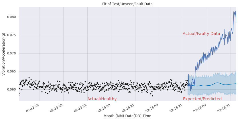
Introduction
Towards Multi Sensor approach
Softwares / Packages Used
The Data Set
Loading Dataset from G.Cloud
The dataset cited above is downloaded and saved to G.Cloud account. Requires password validation for access to data stored in G.Cloud
def load_dataset() :

  """
  Loads datset from  G.Drive
  Arguments:
  Nil
  Returns:
  Nil
  """
  # Install the PyDrive wrapper & import libraries.
  # This only needs to be done once per notebook.
  !pip install -U -q PyDrive
  from pydrive.auth import GoogleAuth
  from pydrive.drive import GoogleDrive
  from google.colab import auth
  from oauth2client.client import GoogleCredentials

  # Authenticate and create the PyDrive client.
  # This only needs to be done once per notebook.
  auth.authenticate_user()
  gauth = GoogleAuth()
  gauth.credentials = GoogleCredentials.get_application_default()
  drive = GoogleDrive(gauth)

  # Download a file based on its file ID
  file_id = '1DaCt511APQoQghiUIUruK7iGrnALkCg6'
  download = drive.CreateFile({'id': file_id})
  download.GetContentFile('data.zip')
  # Unzipping the data file
  !unzip data.zip
  print('Downloaded Data Files & Saved to Local Instance')

load_dataset()
[K |████████████████████████████████| 993kB 2.8MB/s
[?25h Building wheel for PyDrive (setup.py) ... [?25l[?25hdone
Archive: data.zip
inflating: Damage Propagation Modeling.pdf
inflating: readme.txt
inflating: RUL_FD001.txt
inflating: RUL_FD002.txt
inflating: RUL_FD003.txt
inflating: RUL_FD004.txt
inflating: test_FD001.txt
inflating: test_FD002.txt
inflating: test_FD003.txt
inflating: test_FD004.txt
inflating: train_FD001.txt
inflating: train_FD002.txt
inflating: train_FD003.txt
inflating: train_FD004.txt
Downloaded Data Files & Saved to Local Instance
Data Wrangling
import pandas as pd
import numpy as np
import matplotlib.pyplot as plt
import os
from sklearn import preprocessing
from sklearn.metrics import confusion_matrix, recall_score, precision_score

np.random.seed(1)
from keras.models import Model
from keras.layers import Dense, Input, Dropout, LSTM, Activation
from keras.layers.embeddings import Embedding
from keras.preprocessing import sequence
from keras.initializers import glorot_uniform
import tensorflow as tf
from keras.models import load_model
from keras.optimizers import Adam
Using TensorFlow backend.
def to_df_data(filename) :
  """
  Covert to dataframe with proper annotation
  Arguments:
  Nil
  Returns:
  train_data
  """
  data = pd.read_csv(filename, sep=" ", header=None)
  # Dropping the NAN Columns
  data.drop(data.columns[[26, 27]], axis=1, inplace=True)
  # Annotating the Columns
  data.columns = ['id', 'cycle', 'setting1', 'setting2', 'setting3', 's1', 's2', 's3',
                       's4', 's5', 's6', 's7', 's8', 's9', 's10', 's11', 's12', 's13', 's14',
                       's15', 's16', 's17', 's18', 's19', 's20', 's21']
  data = data.sort_values(['id','cycle'])
  return data
Read in Training Data Set
train_data = to_df_data('train_FD001.txt')
train_data.head()
| id | cycle | setting1 | setting2 | setting3 | s1 | s2 | s3 | s4 | s5 | s6 | s7 | s8 | s9 | s10 | s11 | s12 | s13 | s14 | s15 | s16 | s17 | s18 | s19 | s20 | s21 | |
|---|---|---|---|---|---|---|---|---|---|---|---|---|---|---|---|---|---|---|---|---|---|---|---|---|---|---|
| 0 | 1 | 1 | -0.0007 | -0.0004 | 100.0 | 518.67 | 641.82 | 1589.70 | 1400.60 | 14.62 | 21.61 | 554.36 | 2388.06 | 9046.19 | 1.3 | 47.47 | 521.66 | 2388.02 | 8138.62 | 8.4195 | 0.03 | 392 | 2388 | 100.0 | 39.06 | 23.4190 |
| 1 | 1 | 2 | 0.0019 | -0.0003 | 100.0 | 518.67 | 642.15 | 1591.82 | 1403.14 | 14.62 | 21.61 | 553.75 | 2388.04 | 9044.07 | 1.3 | 47.49 | 522.28 | 2388.07 | 8131.49 | 8.4318 | 0.03 | 392 | 2388 | 100.0 | 39.00 | 23.4236 |
| 2 | 1 | 3 | -0.0043 | 0.0003 | 100.0 | 518.67 | 642.35 | 1587.99 | 1404.20 | 14.62 | 21.61 | 554.26 | 2388.08 | 9052.94 | 1.3 | 47.27 | 522.42 | 2388.03 | 8133.23 | 8.4178 | 0.03 | 390 | 2388 | 100.0 | 38.95 | 23.3442 |
| 3 | 1 | 4 | 0.0007 | 0.0000 | 100.0 | 518.67 | 642.35 | 1582.79 | 1401.87 | 14.62 | 21.61 | 554.45 | 2388.11 | 9049.48 | 1.3 | 47.13 | 522.86 | 2388.08 | 8133.83 | 8.3682 | 0.03 | 392 | 2388 | 100.0 | 38.88 | 23.3739 |
| 4 | 1 | 5 | -0.0019 | -0.0002 | 100.0 | 518.67 | 642.37 | 1582.85 | 1406.22 | 14.62 | 21.61 | 554.00 | 2388.06 | 9055.15 | 1.3 | 47.28 | 522.19 | 2388.04 | 8133.80 | 8.4294 | 0.03 | 393 | 2388 | 100.0 | 38.90 | 23.4044 |
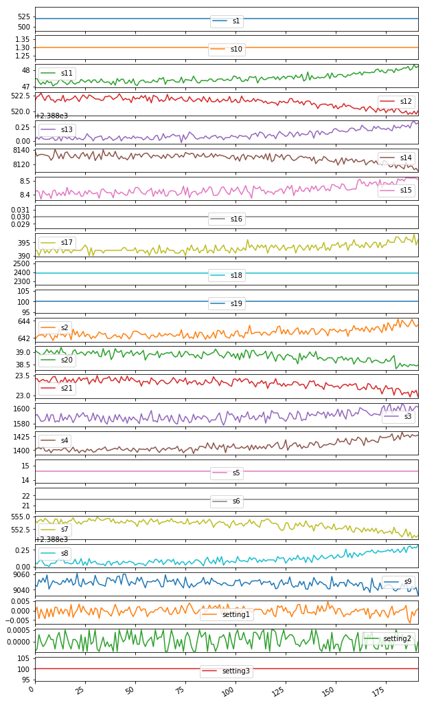
Visualizing Sensor Data
train_data_1 = train_data[train_data['id'] == 1]
plt = train_data_1[train_data_1.columns.difference(['id','cycle'])].plot(subplots=True, sharex=True, figsize=(10,20))
Calculation of Residual Useful Life for Training Data
The dataset is formatted as an end of cycle dataset. First, we need to find the maximum cycle for each engine. Then at any point point the residual useful life is maximum cycle less current cycle number.
def cal_rul(data):
  """
  Calculate RUL from Cycle Column for each Engine
  Arguments:
  Nil
  Returns:
  train_data
  """

  maxlife = pd.DataFrame(data.groupby('id')['cycle'].max()).reset_index()
  maxlife.columns = ['id', 'max']
  data = data.merge(maxlife, on=['id'], how='left')
  rul = pd.DataFrame(data['max'] - data['cycle']).reset_index()
  rul.columns = ['No', 'rul']
  rul['id'] = data['id']

  return maxlife, rul
maxlife, rul_data = cal_rul(train_data)
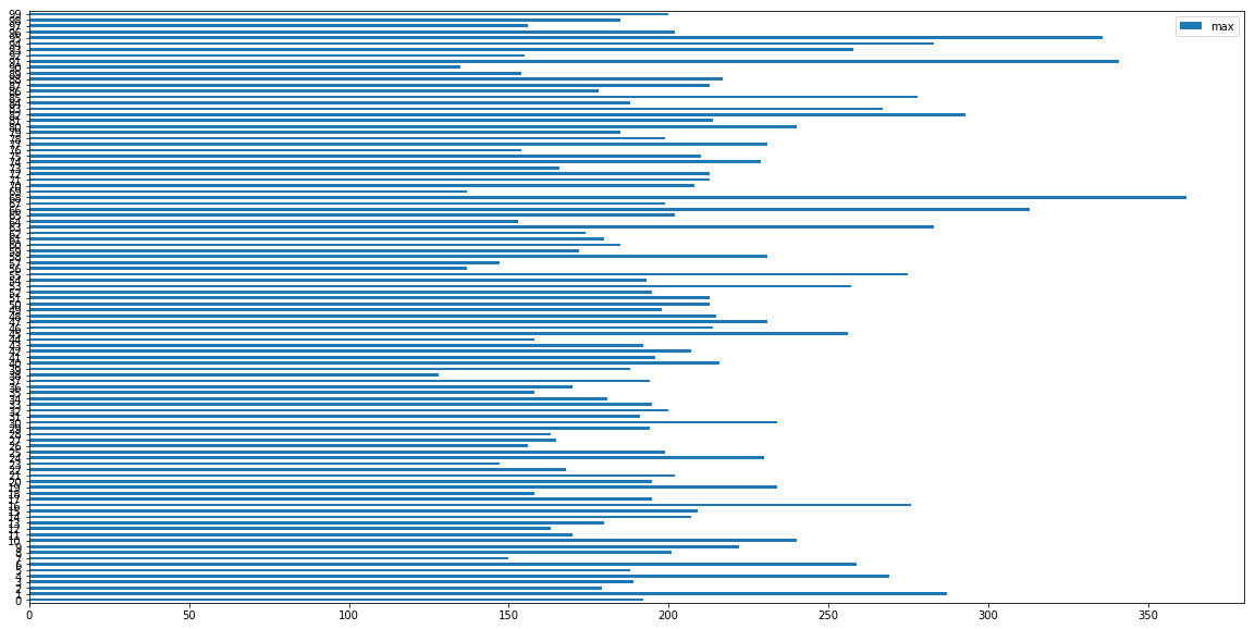
Analysis of life of 100 Engines used in Training Data
# Plot of life of 100 Engines
ax = maxlife.plot.barh(y='max', figsize=(20,10))
print('Max Life of Engines in hours/cycles (out of 100 engines in dataset):' ,  maxlife['max'].max())
print('Min Life of Engines in hours/cycles (out of 100 engines in dataset) :' ,  maxlife['max'].min())
print('Average Life of Engines in hours/cycles (out of 100 engines in dataset) :' ,  maxlife['max'].mean())
Max Life of Engines in hours/cycles (out of 100 engines in dataset): 362
Min Life of Engines in hours/cycles (out of 100 engines in dataset) : 128
Average Life of Engines in hours/cycles (out of 100 engines in dataset) : 206.31
Binary Encoding
Logic : If life left is less than 30 cycles, the output should be “1” else “0”
def predictor_var(rul_data, w) :
  """
  Binary encoding for data
  Same function used for training and test data
  Arguments:
  rul, w=30 cycles
  Returns:
  Y (Dependent Variable)
  """
  Y = pd.DataFrame(np.where(rul_data['rul'] <= w, 1, 0 )).reset_index()
  Y.columns = ['id', 'label']
  Y['id'] = rul_data['id']
  return Y
Binary Encoding for Training Data
Y_train_hot = predictor_var(rul_data, 30)
Normalization
Since we are using mutidimensional data, it is importtant to get them on the same scale. Ensuring standardised feature values implicitly weights all features equally in their representation.
def normalize(data) :
  """
  Binary encoding for data
  Same function used for training and test data
  Arguments:
  data
  Returns:
  X (Independent Variables/Features)
  """

  # train_data['cycle_norm'] = train_data['cycle']
  cols_normalize = data.columns.difference(['id','cycle'])
  min_max_scaler = preprocessing.MinMaxScaler()
  X  = pd.DataFrame(min_max_scaler.fit_transform(data[cols_normalize]),
                               columns=cols_normalize,
                               index=data.index)

  X['id'] = data['id']
  return X
Normalization of Training Data
X_train = normalize(train_data)
Generation of Sequence Data (Independent Variables/Features -X)
A windowing approach is used to generate samples., i.e. first look at 1 to n seq-length, then the next 2 to n seq-length + 1.
Further tf/keras, accepts tenensors in the format (samples, time, features)
# Window Size
sequence_length = 30

def X_sequence(data) :
  """
  Generation of Sequence of X
  Same function used for training and test data
  Arguments:
  data
  Returns:
  Xseq (Sequence of Independent Variables/Features)
  """

  # Reshape features into (samples, time steps, features)
  def gen_sequence(id_df, seq_length, seq_cols):
      # for one id I put all the rows in a single matrix
      data_matrix = id_df[seq_cols].values
      num_elements = data_matrix.shape[0]
      for start, stop in zip(range(0, num_elements-seq_length), range(seq_length, num_elements)):
          yield data_matrix[start:stop, :]

  # Pick the feature columns,(Discard id column)
  sequence_cols = data.columns.difference(['id'])

  # Generator for the sequences
  seq_gen = (list(gen_sequence(data[data['id']==id], sequence_length, sequence_cols))
             for id in data['id'].unique())

  # Generate sequences and convert to numpy array
  Xseq = np.concatenate(list(seq_gen)).astype(np.float32)

  return Xseq
Generation of Sequence Data from Training Set (Independent Variables/Features -X)
Xseq_train = X_sequence(X_train)
print("Shape of Training Data X", Xseq_train.shape)
# (No of samples, window size, Features)
Shape of Training Data X (17631, 30, 24)
Generation of Sequence Data (Dependent Variable - Y)
def Y_sequence(data) :

  def gen_labels(id_df, seq_length, label):
    """
    Generation of Sequence of Y
    Same function used for training and test data
    Arguments:
    data
    Returns:
    Rseq (Sequence of Dependent Variables/Predictor)
    """
    data_matrix = id_df[label].values
    num_elements = data_matrix.shape[0]
    # I have to remove the first seq_length labels
    # because for one id the first sequence of seq_length size have as target
    # the last label (the previus ones are discarded).
    # All the next id's sequences will have associated step by step one label as target.
    return data_matrix[seq_length:num_elements, :]

  # generate labels
  label_gen = [gen_labels(data[data['id']==id], sequence_length, ['label'])
                 for id in data['id'].unique()]
  Y_seq = np.concatenate(label_gen).astype(np.float32)

  return Y_seq
Yseq_train = Y_sequence(Y_train_hot)
print("Shape of Training Data Labels Y", Yseq_train.shape)
Shape of Training Data Labels Y (17631, 1)
Read in Test Set - (Independent Variables/Features X)
# Read and convert to dataframe with prpoer annotations
test_data = to_df_data('test_FD001.txt')
test_data.head()
| id | cycle | setting1 | setting2 | setting3 | s1 | s2 | s3 | s4 | s5 | s6 | s7 | s8 | s9 | s10 | s11 | s12 | s13 | s14 | s15 | s16 | s17 | s18 | s19 | s20 | s21 | |
|---|---|---|---|---|---|---|---|---|---|---|---|---|---|---|---|---|---|---|---|---|---|---|---|---|---|---|
| 0 | 1 | 1 | 0.0023 | 0.0003 | 100.0 | 518.67 | 643.02 | 1585.29 | 1398.21 | 14.62 | 21.61 | 553.90 | 2388.04 | 9050.17 | 1.3 | 47.20 | 521.72 | 2388.03 | 8125.55 | 8.4052 | 0.03 | 392 | 2388 | 100.0 | 38.86 | 23.3735 |
| 1 | 1 | 2 | -0.0027 | -0.0003 | 100.0 | 518.67 | 641.71 | 1588.45 | 1395.42 | 14.62 | 21.61 | 554.85 | 2388.01 | 9054.42 | 1.3 | 47.50 | 522.16 | 2388.06 | 8139.62 | 8.3803 | 0.03 | 393 | 2388 | 100.0 | 39.02 | 23.3916 |
| 2 | 1 | 3 | 0.0003 | 0.0001 | 100.0 | 518.67 | 642.46 | 1586.94 | 1401.34 | 14.62 | 21.61 | 554.11 | 2388.05 | 9056.96 | 1.3 | 47.50 | 521.97 | 2388.03 | 8130.10 | 8.4441 | 0.03 | 393 | 2388 | 100.0 | 39.08 | 23.4166 |
| 3 | 1 | 4 | 0.0042 | 0.0000 | 100.0 | 518.67 | 642.44 | 1584.12 | 1406.42 | 14.62 | 21.61 | 554.07 | 2388.03 | 9045.29 | 1.3 | 47.28 | 521.38 | 2388.05 | 8132.90 | 8.3917 | 0.03 | 391 | 2388 | 100.0 | 39.00 | 23.3737 |
| 4 | 1 | 5 | 0.0014 | 0.0000 | 100.0 | 518.67 | 642.51 | 1587.19 | 1401.92 | 14.62 | 21.61 | 554.16 | 2388.01 | 9044.55 | 1.3 | 47.31 | 522.15 | 2388.03 | 8129.54 | 8.4031 | 0.03 | 390 | 2388 | 100.0 | 38.99 | 23.4130 |
Read in Test Set - (Dependent Variables/Predictor Y)
# Read ground truth data
Yrul_test = pd.read_csv('RUL_FD001.txt', sep=" ", header=None)
Yrul_test.drop(Yrul_test.columns[[1]], axis=1, inplace=True)
Yrul_test.columns = ['cyclesleft']
Yrul_test['id'] = Yrul_test.index + 1
# Find max cycles
X_test_max = pd.DataFrame(test_data.groupby('id')['cycle'].max()).reset_index()
X_test_max.columns = ['id', 'max']
Yrul_test['max'] = X_test_max['max'] + Yrul_test['cyclesleft']
Yrul_test.drop('cyclesleft', axis=1, inplace=True)

# Generate RUL
temp = test_data.merge(Yrul_test, on=['id'], how='left')
Y_test = pd.DataFrame(temp['max'] - temp['cycle']).reset_index()
Y_test.columns = ['No', 'rul']
Y_test['id'] = test_data['id']
Sanity Check of combined dataframe of Test Set
print('Max Life of Engines in hours/cycles (out of 100 engines in dataset):' ,  Yrul_test['max'].max())
print('Min Life of Engines in hours/cycles (out of 100 engines in dataset) :' ,  Yrul_test['max'].min())
print('Average Life of Engines in hours/cycles (out of 100 engines in dataset) :' ,  Yrul_test['max'].mean())
Max Life of Engines in hours/cycles (out of 100 engines in dataset): 341
Min Life of Engines in hours/cycles (out of 100 engines in dataset) : 141
Average Life of Engines in hours/cycles (out of 100 engines in dataset) : 206.48
Normalization of Test Data
X_test = normalize(test_data)
Binary Encoding for Test Data
Y_test_hot = predictor_var(Y_test, 30)
Generation of Sequence Data from Test Set (Independent Variables/ Features -X)
Xseq_test = X_sequence(X_test)
print("Shape of Test Data X", Xseq_test.shape)
Shape of Test Data X (10096, 30, 24)
Generation of Sequence Data from Test Set (Dependent Variable/ Predictor - Y)
Yseq_test = Y_sequence(Y_test_hot)
print("Shape of Test Data Labels Y", Yseq_test.shape)
Shape of Test Data Labels Y (10096, 1)
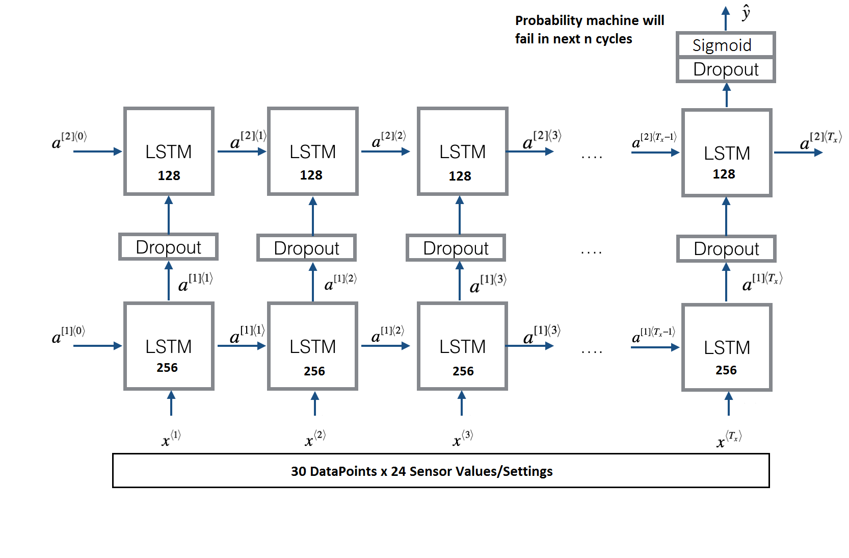
Deep Neural Network Model
# define path to save model
model_path = 'binary_model.h5'

class myCallbacks(tf.keras.callbacks.Callback):
  def on_epoch_end(self, epoch, logs={}):
    if(logs.get('acc') > 0.99):
      print("\n Reached training accuracy of 99%")
      self.model.stop_training = True
def LSTM_model(input_shape):
    """
    Function creating the model graph.

    Arguments:
    input_shape -- shape of the input

    Returns:
    model -- a model instance in Keras
    """
    X_input = Input(shape = input_shape)

    # Propagate the inputs through an LSTM layer with 256-dimensional hidden state
    X = LSTM(256, return_sequences=True)(X_input)
    # Add dropout with a probability of 0.5
    X = Dropout(0.5)(X)
    # Propagate the inputs through an LSTM layer with 128-dimensional hidden state
    X = LSTM(128, return_sequences=False)(X)
    # Add dropout with a probability of 0.5
    X = Dropout(0.5)(X)
    # Propagate X through a Dense layer with softmax activation to get back a batch of 2-dimensional vectors.
    X = Dense(1)(X)
    # Add a softmax activation
    X = Activation('sigmoid')(X)

    # Create Model instance which converts sentence_indices into X.
    model = Model(input=X_input, output=X)

    ### END CODE HERE ###

    return model
input_shape = (Xseq_train.shape[1], Xseq_train.shape[2])
model = LSTM_model(input_shape)
WARNING: Logging before flag parsing goes to stderr.
W0803 04:44:51.141316 140401135368064 deprecation_wrapper.py:119] From /usr/local/lib/python3.6/dist-packages/keras/backend/tensorflow_backend.py:74: The name tf.get_default_graph is deprecated. Please use tf.compat.v1.get_default_graph instead.

W0803 04:44:51.183787 140401135368064 deprecation_wrapper.py:119] From /usr/local/lib/python3.6/dist-packages/keras/backend/tensorflow_backend.py:517: The name tf.placeholder is deprecated. Please use tf.compat.v1.placeholder instead.

W0803 04:44:51.194183 140401135368064 deprecation_wrapper.py:119] From /usr/local/lib/python3.6/dist-packages/keras/backend/tensorflow_backend.py:4138: The name tf.random_uniform is deprecated. Please use tf.random.uniform instead.

W0803 04:44:51.547616 140401135368064 deprecation_wrapper.py:119] From /usr/local/lib/python3.6/dist-packages/keras/backend/tensorflow_backend.py:133: The name tf.placeholder_with_default is deprecated. Please use tf.compat.v1.placeholder_with_default instead.

W0803 04:44:51.559854 140401135368064 deprecation.py:506] From /usr/local/lib/python3.6/dist-packages/keras/backend/tensorflow_backend.py:3445: calling dropout (from tensorflow.python.ops.nn_ops) with keep_prob is deprecated and will be removed in a future version.
Instructions for updating:
Please use `rate` instead of `keep_prob`. Rate should be set to `rate = 1 - keep_prob`.
/usr/local/lib/python3.6/dist-packages/ipykernel_launcher.py:27: UserWarning: Update your `Model` call to the Keras 2 API: `Model(inputs=Tensor("in..., outputs=Tensor("ac...)`
model.summary()
_________________________________________________________________
Layer (type)                 Output Shape              Param #
=================================================================
input_1 (InputLayer)         (None, 30, 24)            0
_________________________________________________________________
lstm_1 (LSTM)                (None, 30, 256)           287744
_________________________________________________________________
dropout_1 (Dropout)          (None, 30, 256)           0
_________________________________________________________________
lstm_2 (LSTM)                (None, 128)               197120
_________________________________________________________________
dropout_2 (Dropout)          (None, 128)               0
_________________________________________________________________
dense_1 (Dense)              (None, 1)                 129
_________________________________________________________________
activation_1 (Activation)    (None, 1)                 0
=================================================================
Total params: 484,993
Trainable params: 484,993
Non-trainable params: 0
_________________________________________________________________
def run_model() :
    """
    Compiles and run the model

    Arguments:
    Nil

    Returns:
    histroy - dict_keys(['val_loss', 'val_acc', 'loss', 'acc'])
    """
  opt = Adam(lr = 0.0001, beta_1 = 0.9, beta_2 = 0.999, decay = 0.01)
  model.compile(loss='binary_crossentropy', optimizer= opt, metrics=['accuracy'])
  history = model.fit(Xseq_train, Yseq_train, epochs=20, batch_size=200, validation_split=0.05, verbose=2)
  return history


# Following to be run only if model is to be compiled, else, load saved model for testing; Uncomment as necessary
history = run_model()
# model.save(model_path)
Train on 16749 samples, validate on 882 samples
Epoch 1/20
 - 54s - loss: 0.0956 - acc: 0.9602 - val_loss: 0.0690 - val_acc: 0.9671
Epoch 2/20
 - 52s - loss: 0.0820 - acc: 0.9645 - val_loss: 0.0667 - val_acc: 0.9637
Epoch 3/20
 - 52s - loss: 0.0817 - acc: 0.9649 - val_loss: 0.0740 - val_acc: 0.9569
Epoch 4/20
 - 51s - loss: 0.0801 - acc: 0.9654 - val_loss: 0.0663 - val_acc: 0.9637
Epoch 5/20
 - 51s - loss: 0.0789 - acc: 0.9651 - val_loss: 0.0692 - val_acc: 0.9694
Epoch 6/20
 - 51s - loss: 0.0807 - acc: 0.9647 - val_loss: 0.0723 - val_acc: 0.9637
Epoch 7/20
 - 51s - loss: 0.0796 - acc: 0.9657 - val_loss: 0.0651 - val_acc: 0.9649
Epoch 8/20
 - 51s - loss: 0.0776 - acc: 0.9662 - val_loss: 0.0632 - val_acc: 0.9660
Epoch 9/20
 - 52s - loss: 0.0768 - acc: 0.9667 - val_loss: 0.0670 - val_acc: 0.9626
Epoch 10/20
 - 52s - loss: 0.0795 - acc: 0.9650 - val_loss: 0.0672 - val_acc: 0.9671
Epoch 11/20
 - 52s - loss: 0.0767 - acc: 0.9668 - val_loss: 0.0705 - val_acc: 0.9637
Epoch 12/20
 - 52s - loss: 0.0793 - acc: 0.9660 - val_loss: 0.0689 - val_acc: 0.9649
Epoch 13/20
 - 52s - loss: 0.0761 - acc: 0.9675 - val_loss: 0.0713 - val_acc: 0.9626
Epoch 14/20
 - 52s - loss: 0.0752 - acc: 0.9669 - val_loss: 0.0655 - val_acc: 0.9637
Epoch 15/20
 - 52s - loss: 0.0766 - acc: 0.9656 - val_loss: 0.0672 - val_acc: 0.9626
Epoch 16/20
 - 52s - loss: 0.0755 - acc: 0.9669 - val_loss: 0.0706 - val_acc: 0.9626
Epoch 17/20
 - 52s - loss: 0.0760 - acc: 0.9666 - val_loss: 0.0666 - val_acc: 0.9615
Epoch 18/20
 - 52s - loss: 0.0754 - acc: 0.9679 - val_loss: 0.0642 - val_acc: 0.9660
Epoch 19/20
 - 52s - loss: 0.0755 - acc: 0.9676 - val_loss: 0.0629 - val_acc: 0.9649
Epoch 20/20
 - 52s - loss: 0.0759 - acc: 0.9676 - val_loss: 0.0623 - val_acc: 0.9649
# model = load_model(model_path)
Measuring Accuracy of Model
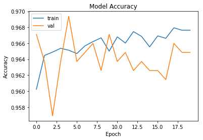
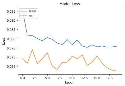
The model trained above is evaluated on a test set. Plot of accuracy and loss is observed to check overfitting and track overall performace. Confusion matrix and accracy measures for a binary model like precision, recall and F1 score is put up.
Evaluation on Test Set
loss, acc = model.evaluate(Xseq_test, Yseq_test)
print("Test Set Accuracy = ", acc)
10096/10096 [==============================] - 9s 882us/step
Test Set Accuracy =  0.9117472266244057
Plot of model accuracy and loss
import matplotlib.pyplot as plt
# Accuracy Plots
plt.plot(history.history['acc'])
plt.plot(history.history['val_acc'])
plt.title('Model Accuracy')
plt.ylabel('Accuracy')
plt.xlabel('Epoch')
plt.legend(['train', 'val'], loc='upper left')
plt.show()
# Loss plots
plt.plot(history.history['loss'])
plt.plot(history.history['val_loss'])
plt.title('Model Loss')
plt.ylabel('Loss')
plt.xlabel('Epoch')
plt.legend(['train', 'val'], loc='upper left')
plt.show()
Confusion Matrix
Note that the probability measure is a hyperparamter and should be adjusted to get the desired values of precision and recall as per system requirments.
# Make predictions and compute confusion matrix
y_pred_prob = model.predict(Xseq_test)
y_pred = y_pred_prob > 0.99
y_true = Yseq_test
print('Confusion matrix\n- x-axis is true labels.\n- y-axis is predicted labels')
cm = confusion_matrix(y_true, y_pred)
print(cm)

# Compute precision and recall
precision = precision_score(y_true, y_pred)
recall = recall_score(y_true, y_pred)
f1 = 2 * (precision * recall) / (precision + recall)
print( ' Precision: ', precision, '\n', 'Recall: ', recall,'\n', 'F1-score:', f1 )
Confusion matrix
- x-axis is true labels.
- y-axis is predicted labels
[[9485  279]
 [  49  283]]
 Precision:  0.50355871886121
 Recall:  0.8524096385542169
 F1-score: 0.6331096196868009
# Helper commands for creating plot in demo
'''
import sys
numpy.set_printoptions(threshold=sys.maxsize)
Xseq_test[0:2]
y_pred_prob[80]
import matplotlib.pyplot as plt
plt.plot(y_pred_prob[0:80])
t = y_pred_prob[843:1015].T*100
t = y_pred_prob[0:80].T*100
a= t[0]
y=np.arange(a.shape[0])
np.vstack((y,a))
'''
Conclusion
An F1 score of 0.633 is to be treated as baseline only. Future posts will delve into improvements in the model.
References
- https://datascientistinabox.com/2015/11/30/predictive-modeling-of-turbofan-degradation-part-1/
- https://github.com/hankroark/Turbofan-Engine-Degradation/blob/master/models/Turbofan-Degradation-DataSet-FD001.ipynb
- https://github.com/umbertogriffo/Predictive-Maintenance-using-LSTM
- https://www.ncbi.nlm.nih.gov/pmc/articles/PMC6068676/ 5.https://archive.ics.uci.edu/ml/datasets/Condition+monitoring+of+hydraulic+systems
- https://www.adb.org/sites/default/files/publication/350011/sdwp-48.pdf
- https://c3.ai/customers/engie/
- Andrew Ng, Deep Learning Specialization, Coursera
- http://colah.github.io/posts/2015-08-Understanding-LSTMs/